Introduction
Traditional keyword search has a fundamental limitation: it can only match exact words. Search for “happy” and you won’t find documents containing “joyful,” “delighted,” or “cheerful”—despite their semantic similarity.
Vector embeddings solve this problem by representing text as points in a high-dimensional space where semantic meaning determines distance. Words, sentences, or entire documents with similar meanings cluster together, enabling truly semantic search.
This technology underpins nearly every modern AI application:
- Search engines: Understanding query intent beyond keywords.
- Recommendation systems: Finding similar content based on meaning.
- LLM applications: Retrieval-Augmented Generation (RAG).
- Question answering: Matching questions to relevant answers.
- Duplicate detection: Finding semantically identical content.
In this post, we’ll explore how embeddings work, from classical approaches like word2vec to modern transformer-based methods, and how to implement semantic search at scale using vector databases like Elasticsearch.
What Are Embeddings?
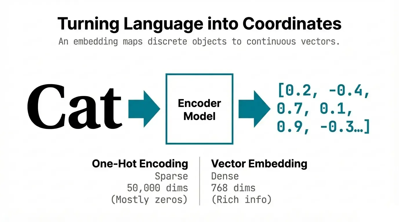
An embedding is a learned representation that maps discrete objects (words, sentences, images) to continuous vectors in a way that captures semantic relationships.
The Core Idea
# Traditional representation (one-hot encoding)
"cat"  = [1, 0, 0, 0, ..., 0]  # 50,000 dimensions, sparse
"dog"  = [0, 1, 0, 0, ..., 0]
"car"  = [0, 0, 1, 0, ..., 0]

# Embedding representation (dense vectors)
"cat"  = [0.2, -0.4, 0.7, 0.1, ...]  # 768 dimensions, dense
"dog"  = [0.3, -0.3, 0.8, 0.0, ...]  # Similar to cat
"car"  = [0.8, 0.5, -0.2, 0.9, ...]  # Different from cat/dog
Key properties:
- Dense: Most values are non-zero.
- Low-dimensional: Typically 128-1536 dimensions vs millions for one-hot.
- Semantic: Similar meanings → similar vectors.
- Learned: Trained from data, not hand-crafted.
Word2Vec: The Breakthrough (2013)
The Distributional Hypothesis
“You shall know a word by the company it keeps” — J.R. Firth (1957)
Word2Vec, introduced by Mikolov et al. at Google, operationalized this idea: words appearing in similar contexts have similar meanings.
Two Architectures
1. CBOW (Continuous Bag of Words)
Predict the center word from surrounding context:
Context: "The cat sat on the ___"
Target:  "mat"

Input:  [the, cat, sat, on, the] → Average embeddings
Output: Predict "mat"
2. Skip-gram
Predict context words from center word (more popular):
Target:  "cat"
Output:  Predict context words: [the, sat, on, mat]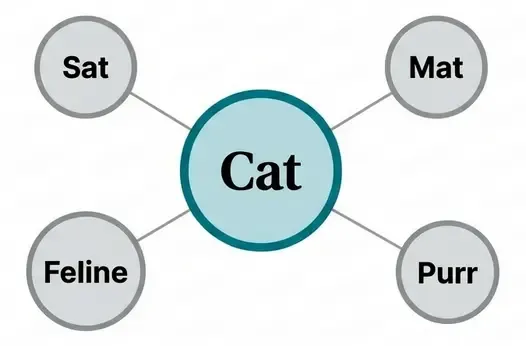
Skip-gram Implementation
import torch
import torch.nn as nn

class SkipGramModel(nn.Module):
    def __init__(self, vocab_size, embedding_dim):
        super().__init__()
        self.embedding = nn.Embedding(vocab_size, embedding_dim)
        self.output = nn.Linear(embedding_dim, vocab_size)

    def forward(self, target_word):
        # Get embedding for target word
        embedded = self.embedding(target_word)

        # Predict context words
        output = self.output(embedded)
        return output

# Training
vocab_size = 10000
embedding_dim = 300

model = SkipGramModel(vocab_size, embedding_dim)
criterion = nn.CrossEntropyLoss()
optimizer = torch.optim.Adam(model.parameters())

# Training loop
for target_word, context_words in training_pairs:
    optimizer.zero_grad()

    # Forward pass
    predictions = model(target_word)

    # Loss for each context word
    loss = sum(criterion(predictions, context_word)
               for context_word in context_words)

    loss.backward()
    optimizer.step()
Optimization: Negative Sampling
Training on all vocabulary words is expensive. Negative sampling trains on:
- Positive pairs: (target, actual context).
- Negative pairs: (target, random words).
def negative_sampling_loss(target_emb, positive_emb, negative_embs):
    """
    Maximize: sigmoid(target · positive)
    Minimize: sigmoid(target · negative_i)
    """
    # Positive sample
    positive_score = torch.sigmoid(torch.dot(target_emb, positive_emb))
    positive_loss = -torch.log(positive_score)

    # Negative samples
    negative_scores = torch.sigmoid(torch.matmul(negative_embs, target_emb))
    negative_loss = -torch.sum(torch.log(1 - negative_scores))

    return positive_loss + negative_loss
Remarkable Properties
Word2Vec embeddings exhibit semantic and syntactic relationships:
# Vector arithmetic
king - man + woman ≈ queen
paris - france + spain ≈ madrid
walking - walk + swim ≈ swimming

# Similarity
cosine_similarity("king", "queen")   # High (~0.7)
cosine_similarity("king", "car")     # Low (~0.1)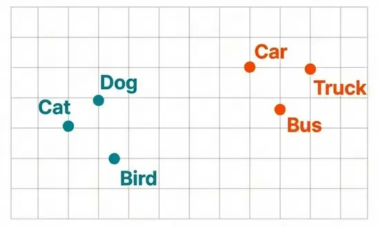
From Words to Sentences: Evolution of Embeddings
Limitation of Word2Vec
Word2Vec produces fixed embeddings: each word has one vector regardless of context.
# "bank" has same embedding in both:
"I went to the bank to withdraw money"      # financial institution
"I sat on the river bank to relax"          # riverbank
GloVe (2014): Global Vectors
Combines global matrix factorization with local context:
# Objective: embedding should reflect co-occurrence statistics
J = Σ f(X_ij) * (w_i · w_j + b_i + b_j - log(X_ij))²

where:
- X_ij = co-occurrence count of word i and j.
- w_i, w_j = word vectors.
- f(X_ij) = weighting function (more weight to frequent pairs).
ELMo (2018): Context-Aware Embeddings
First contextualized embeddings using bidirectional LSTMs:
# Different embeddings based on context
embedding_1 = elmo("I went to the bank to withdraw")
embedding_2 = elmo("I sat on the river bank")

# embedding_1["bank"] ≠ embedding_2["bank"]
Transformer-Based Embeddings: State of the Art
BERT Embeddings (2018+)
BERT and its variants produce contextualized embeddings through self-attention:
from transformers import BertModel, BertTokenizer

model = BertModel.from_pretrained('bert-base-uncased')
tokenizer = BertTokenizer.from_pretrained('bert-base-uncased')

text = "The cat sat on the mat"
inputs = tokenizer(text, return_tensors='pt')

# Get embeddings
with torch.no_grad():
    outputs = model(**inputs)

# Different embedding strategies:
# 1. Last layer [CLS] token (sentence embedding)
cls_embedding = outputs.last_hidden_state[:, 0, :]  # [1, 768]

# 2. Mean pooling of all tokens
token_embeddings = outputs.last_hidden_state  # [1, seq_len, 768]
attention_mask = inputs['attention_mask']
mean_embedding = torch.sum(token_embeddings * attention_mask.unsqueeze(-1), dim=1)
mean_embedding = mean_embedding / torch.sum(attention_mask, dim=1, keepdim=True)

# 3. Max pooling
max_embedding = torch.max(token_embeddings, dim=1)[0]
Sentence Transformers (2019)
BERT wasn’t optimized for semantic similarity. Sentence-BERT (SBERT) fine-tunes BERT specifically for producing semantically meaningful sentence embeddings.
Architecture:
       Input Sentences
            ↓
   ┌────────────────────┐
   │  BERT / RoBERTa    │
   │  (shared weights)  │
   └────────┬───────────┘
            ↓
      Mean Pooling
            ↓
     Normalization
            ↓
   Sentence Embedding
      (768 dimensions)
Training with Siamese Networks:
from sentence_transformers import SentenceTransformer, losses
from torch.utils.data import DataLoader

model = SentenceTransformer('bert-base-uncased')

# Training data: (sentence1, sentence2, similarity_score)
train_examples = [
    ("The cat sits on the mat", "A feline rests on a rug", 0.8),
    ("I love pizza", "The weather is nice", 0.1),
    ("He plays soccer", "She enjoys football", 0.7),
]

# Convert to DataLoader
train_dataloader = DataLoader(train_examples, shuffle=True, batch_size=16)

# Cosine similarity loss
train_loss = losses.CosineSimilarityLoss(model)

# Train
model.fit(
    train_objectives=[(train_dataloader, train_loss)],
    epochs=1,
    warmup_steps=100
)
Usage:
from sentence_transformers import SentenceTransformer, util

model = SentenceTransformer('all-MiniLM-L6-v2')

# Generate embeddings
sentences = [
    "I love machine learning",
    "I enjoy artificial intelligence",
    "The weather is sunny today"
]

embeddings = model.encode(sentences)

# Compute similarities
similarity_matrix = util.cos_sim(embeddings, embeddings)

print(similarity_matrix)
# [[1.00, 0.72, 0.13],   # "machine learning" most similar to "AI"
#  [0.72, 1.00, 0.15],
#  [0.13, 0.15, 1.00]]
Popular Models (2023)
| Model | Dimensions | Use Case | Performance |
|---|---|---|---|
| all-MiniLM-L6-v2 | 384 | Fast, general purpose | Good |
| all-mpnet-base-v2 | 768 | Better quality | Very good |
| instructor-xl | 768 | Task-specific instructions | Excellent |
| E5-large | 1024 | State-of-the-art | Excellent |
| OpenAI text-embedding-ada-002 | 1536 | Commercial API | Excellent |
2026 Update: State-of-the-Art Models
The embedding landscape has evolved significantly. Modern models now offer better quality, longer context windows, and multilingual capabilities:
| Model | Dimensions | Context Length | Key Features | Performance |
|---|---|---|---|---|
| OpenAI text-embedding-3-large | 3072 (configurable) | 8191 tokens | Best quality, configurable dimensions | Excellent |
| OpenAI text-embedding-3-small | 1536 (configurable) | 8191 tokens | Cost-effective, fast | Very good |
| Cohere embed-v3 | 1024 | 512 tokens | Multilingual (100+ languages), compression | Excellent |
| Voyage-large-2 | 1536 | 16000 tokens | Long context, domain-specific variants | Excellent |
| jina-embeddings-v2-base | 768 | 8192 tokens | Open-source, long context | Very good |
| NV-Embed-v2 | 4096 | 32768 tokens | NVIDIA, longest context | Excellent |
| bge-m3 | 1024 | 8192 tokens | Multi-granularity (dense + sparse + colbert) | Excellent |
| Alibaba GTE-large | 1024 | 512 tokens | Strong on retrieval benchmarks | Very good |
Key trends in 2026:
- Longer context: Models now handle 8K-32K tokens vs 512 in 2023.
- Configurable dimensions: Trade-off between quality and storage (e.g., OpenAI’s matryoshka embeddings).
- Multi-vector representations: Hybrid dense + sparse + late interaction (e.g., BGE-M3).
- Domain specialization: Finance, medical, legal-specific models.
- Better multilingual: True cross-lingual semantic search across 100+ languages.
- Efficiency improvements: 2-3x faster inference with quantization and distillation.
Migration considerations:
- Re-embedding existing corpora with newer models can improve retrieval quality by 10-20%.
- Backward compatibility: Most vector databases support multiple embedding dimensions.
- Cost: OpenAI text-embedding-3-small is 5x cheaper than ada-002 with similar quality.
Similarity Metrics: Measuring Distance
1. Cosine Similarity
Most common for text embeddings:
def cosine_similarity(a, b):
    """
    cos(θ) = (a · b) / (||a|| * ||b||)
    Range: [-1, 1]
    """
    return np.dot(a, b) / (np.linalg.norm(a) * np.linalg.norm(b))

# Example
vec_a = np.array([1, 2, 3])
vec_b = np.array([2, 4, 6])  # Same direction

similarity = cosine_similarity(vec_a, vec_b)
# Output: 1.0 (identical direction)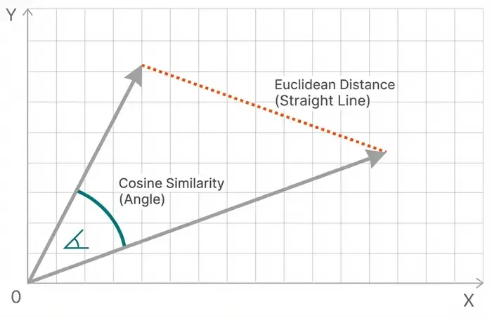
Why cosine?
- Magnitude-invariant (focuses on direction).
- Range [-1, 1] easy to interpret.
- Efficient computation (single dot product).
2. Euclidean Distance
Geometric distance in vector space:
def euclidean_distance(a, b):
    """
    d = √(Σ(a_i - b_i)²)
    Range: [0, ∞)
    """
    return np.sqrt(np.sum((a - b) ** 2))

# Or use numpy
distance = np.linalg.norm(a - b)
When to use:
- Normalized embeddings.
- Clustering algorithms.
- When magnitude matters.
3. Dot Product
Raw similarity without normalization:
def dot_product(a, b):
    """
    a · b = Σ(a_i * b_i)
    Range: (-∞, ∞)
    """
    return np.dot(a, b)
Advantages:
- Fastest computation.
- No square root or division.
- Good for normalized vectors.
4. Manhattan Distance (L1)
Sum of absolute differences:
def manhattan_distance(a, b):
    """
    d = Σ|a_i - b_i|
    """
    return np.sum(np.abs(a - b))
Comparison Example
import numpy as np

# Two embeddings
vec1 = np.array([0.5, 0.8, 0.3])
vec2 = np.array([0.6, 0.7, 0.4])

# Different metrics
cosine = cosine_similarity(vec1, vec2)        # 0.987 (very similar)
euclidean = euclidean_distance(vec1, vec2)    # 0.173 (close)
dot = dot_product(vec1, vec2)                 # 0.98
manhattan = manhattan_distance(vec1, vec2)    # 0.30
Vector Databases: Searching at Scale
The Challenge
With millions of vectors, brute-force search is impractical:
# Brute force: O(n * d) where n = vectors, d = dimensions
def brute_force_search(query, corpus, k=10):
    similarities = []
    for doc_embedding in corpus:  # n iterations
        sim = cosine_similarity(query, doc_embedding)  # d operations
        similarities.append(sim)

    # Return top-k
    top_k_indices = np.argsort(similarities)[-k:]
    return top_k_indices
For 1 million 768-dimensional vectors: ~768 million operations per query ❌
Approximate Nearest Neighbor (ANN) Algorithms
Trade perfect accuracy for massive speed improvements.
1. HNSW (Hierarchical Navigable Small World)
Most popular algorithm (used by Elasticsearch, Pinecone, Weaviate):
Level 2: • ─────────── •
         │             │
Level 1: • ──── • ──── • ──── •
         │      │      │      │
Level 0: •─•─•─•─•─•─•─•─•─•─•  (all vectors)
How it works:
- Build hierarchical graph of vectors.
- Search starts at top level (sparse, long jumps).
- Descend levels, refining search.
- Bottom level has all vectors.
# Simplified HNSW concept
class HNSW:
    def search(self, query, k=10):
        # Start at top level
        current_node = self.entry_point

        for level in range(self.max_level, -1, -1):
            # Greedy search in current level
            while True:
                neighbors = self.get_neighbors(current_node, level)
                closest = min(neighbors, key=lambda n: distance(query, n))

                if distance(query, closest) >= distance(query, current_node):
                    break
                current_node = closest

        # Refined search at level 0
        return self.get_k_nearest(current_node, query, k)
Performance:
- Build time: O(n log n).
- Query time: O(log n).
- Recall: ~95-99% of exact results.
2. IVF (Inverted File Index)
Partition space into clusters:
# IVF concept
from sklearn.cluster import KMeans

class IVF:
    def __init__(self, n_clusters=100):
        self.n_clusters = n_clusters
        self.kmeans = KMeans(n_clusters=n_clusters)

    def build_index(self, vectors):
        # Cluster all vectors
        self.cluster_centers = self.kmeans.fit(vectors)

        # Assign each vector to nearest cluster
        self.inverted_lists = [[] for _ in range(self.n_clusters)]
        for i, vec in enumerate(vectors):
            cluster_id = self.kmeans.predict([vec])[0]
            self.inverted_lists[cluster_id].append((i, vec))

    def search(self, query, k=10, n_probe=5):
        # Find nearest clusters to query
        cluster_distances = [
            (i, distance(query, center))
            for i, center in enumerate(self.cluster_centers)
        ]
        nearest_clusters = sorted(cluster_distances, key=lambda x: x[1])[:n_probe]

        # Search only in nearest clusters
        candidates = []
        for cluster_id, _ in nearest_clusters:
            candidates.extend(self.inverted_lists[cluster_id])

        # Find top-k in candidates
        similarities = [(i, cosine_similarity(query, vec))
                       for i, vec in candidates]
        return sorted(similarities, key=lambda x: x[1], reverse=True)[:k]
3. LSH (Locality-Sensitive Hashing)
Hash similar vectors to same buckets:
# LSH concept
import random
class LSH:
def __init__(self, n_hash_functions=10, n_buckets=1000):
self.n_hash_functions = n_hash_functions
self.hash_tables = [{} for _ in range(n_hash_functions)]
# Random hyperplanes for hashing
self.hyperplanes = [
np.random.randn(embedding_dim)
for _ in range(n_hash_functions)
]
def hash_vector(self, vec, hyperplane):
# Project onto hyperplane, threshold at 0
return int(np.dot(vec, hyperplane) > 0)
def insert(self, vec_id, vec):
for i, hyperplane in enumerate(self.hyperplanes):
hash_val = self.hash_vector(vec, hyperplane)
if hash_val not in self.hash_tables[i]:
self.hash_tables[i][hash_val] = []
self.hash_tables[i][hash_val].append((vec_id, vec))
def search(self, query, k=10):
# Find candidates from all hash tables
candidates = set()
for i, hyperplane in enumerate(self.hyperplanes):
hash_val = self.hash_vector(query, hyperplane)
if hash_val in self.hash_tables[i]:
candidates.update(self.hash_tables[i][hash_val])
# Compute exact similarities for candidates
similarities = [(id, cosine_similarity(query, vec))
for id, vec in candidates]
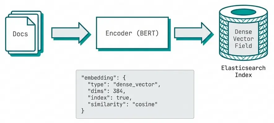
return sorted(similarities, key=lambda x: x[1], reverse=True)[:k]Elasticsearch for Vector Search
Elasticsearch 8.0+ has native vector search support (kNN).
Index Setup
PUT /my-embeddings
{
  "mappings": {
    "properties": {
      "title": {
        "type": "text"
      },
      "content": {
        "type": "text"
      },
      "embedding": {
        "type": "dense_vector",
        "dims": 384,
        "index": true,
        "similarity": "cosine"
      }
    }
  }
}
Indexing Documents
from elasticsearch import Elasticsearch
from sentence_transformers import SentenceTransformer

es = Elasticsearch(['http://localhost:9200'])
model = SentenceTransformer('all-MiniLM-L6-v2')

# Index documents with embeddings
documents = [
    {"title": "Machine Learning Basics", "content": "ML is a subset of AI..."},
    {"title": "Deep Learning Guide", "content": "Neural networks are..."},
    {"title": "NLP Tutorial", "content": "Natural language processing..."}
]

for i, doc in enumerate(documents):
    # Generate embedding
    embedding = model.encode(doc['content']).tolist()

    # Index document
    es.index(
        index='my-embeddings',
        id=i,
        document={
            'title': doc['title'],
            'content': doc['content'],
            'embedding': embedding
        }
    )
Semantic Search Query
def semantic_search(query_text, k=10):
    # Generate query embedding
    query_embedding = model.encode(query_text).tolist()

    # kNN search
    response = es.search(
        index='my-embeddings',
        knn={
            'field': 'embedding',
            'query_vector': query_embedding,
            'k': k,
            'num_candidates': 100  # Number of candidates to consider
        }
    )

    return [hit['_source'] for hit in response['hits']['hits']]

# Query
results = semantic_search("How do neural networks work?")
for doc in results:
    print(f"{doc['title']}: {doc['content'][:100]}...")
Hybrid Search: Combining Dense and Sparse
Best results often come from combining semantic (dense) and keyword (sparse) search:
def hybrid_search(query_text, k=10, dense_weight=0.7):
    query_embedding = model.encode(query_text).tolist()

    response = es.search(
        index='my-embeddings',
        query={
            'bool': {
                'should': [
                    # Semantic search (dense vectors)
                    {
                        'knn': {
                            'field': 'embedding',
                            'query_vector': query_embedding,
                            'k': k,
                            'boost': dense_weight
                        }
                    },
                    # Keyword search (BM25)
                    {
                        'multi_match': {
                            'query': query_text,
                            'fields': ['title^2', 'content'],
                            'boost': 1 - dense_weight
                        }
                    }
                ]
            }
        },
        size=k
    )

    return response['hits']['hits']
Performance Tuning
# Index settings for optimal performance
PUT /my-embeddings
{
  "settings": {
    "index": {
      "number_of_shards": 2,
      "number_of_replicas": 1,
      "knn": true,
      "knn.algo_param.ef_construction": 100  # HNSW build quality
    }
  },
  "mappings": {
    "properties": {
      "embedding": {
        "type": "dense_vector",
        "dims": 384,
        "index": true,
        "similarity": "cosine",
        "index_options": {
          "type": "hnsw",
          "m": 16,           # Number of connections per node
          "ef_construction": 100  # Build-time accuracy
        }
      }
    }
  }
}
Dense vs Sparse Vectors
Dense Vectors
Characteristics:
- Most values are non-zero.
- Learned from neural networks.
- Capture semantic meaning.
- Typical dimensions: 128-1536.
Example:
dense = [0.23, -0.45, 0.12, 0.89, -0.34, ...] # 384 dimensionsAdvantages:
- Capture semantic similarity.
- Generalize to synonyms and paraphrases.
- Work across languages (multilingual models).
Disadvantages:
- Computationally expensive.
- Black box (hard to interpret).
- May miss exact keyword matches.
Sparse Vectors
Characteristics:
- Most values are zero.
- Explicit features (e.g., TF-IDF, BM25).
- Typically very high dimensional.
- Interpretable.
Example:
# TF-IDF vector (vocab size = 50,000)
sparse = {
    4523: 0.8,   # "machine"
    8901: 0.6,   # "learning"
    15234: 0.4   # "algorithm"
}  # Only 3 non-zero values out of 50,000
Advantages:
- Fast exact keyword matching.
- Interpretable (see which words match).
- Good for domain-specific terms.
Disadvantages:
- No semantic understanding.
- Vocabulary mismatch problem.
- Language-specific.
SPLADE: Best of Both Worlds
SPLADE learns sparse vectors using neural networks:
from transformers import AutoModelForMaskedLM, AutoTokenizer

model = AutoModelForMaskedLM.from_pretrained('naver/splade-cocondenser-ensembledistil')
tokenizer = AutoTokenizer.from_pretrained('naver/splade-cocondenser-ensembledistil')

def compute_splade_vector(text):
    inputs = tokenizer(text, return_tensors='pt')

    with torch.no_grad():
        logits = model(**inputs).logits

    # ReLU + log(1 + x) activation
    weights = torch.nn.functional.relu(logits)
    weights = torch.log(1 + weights)

    # Max pooling over tokens
    sparse_vector = torch.max(weights, dim=1).values.squeeze()

    # Keep only top-k dimensions
    top_k = torch.topk(sparse_vector, k=100)

    return {int(idx): float(val) for idx, val in zip(top_k.indices, top_k.values)}
Practical Applications
1. Semantic Search Engine
class SemanticSearchEngine:
    def __init__(self, model_name='all-MiniLM-L6-v2'):
        self.model = SentenceTransformer(model_name)
        self.documents = []
        self.embeddings = None

    def index_documents(self, documents):
        """Index a corpus of documents"""
        self.documents = documents
        self.embeddings = self.model.encode(
            documents,
            convert_to_tensor=True,
            show_progress_bar=True
        )

    def search(self, query, top_k=5):
        """Search for similar documents"""
        query_embedding = self.model.encode(query, convert_to_tensor=True)

        # Compute cosine similarities
        similarities = util.cos_sim(query_embedding, self.embeddings)[0]

        # Get top-k results
        top_results = torch.topk(similarities, k=min(top_k, len(self.documents)))

        results = []
        for score, idx in zip(top_results.values, top_results.indices):
            results.append({
                'document': self.documents[idx],
                'score': float(score),
                'index': int(idx)
            })

        return results

# Usage
engine = SemanticSearchEngine()
engine.index_documents([
    "Python is a programming language",
    "Machine learning is a subset of AI",
    "Deep learning uses neural networks",
    "Natural language processing analyzes text"
])

results = engine.search("What is AI?")
for result in results:
    print(f"Score: {result['score']:.3f} | {result['document']}")
2. Duplicate Detection
def find_duplicates(texts, threshold=0.85):
    """Find semantically similar/duplicate texts"""
    model = SentenceTransformer('all-MiniLM-L6-v2')
    embeddings = model.encode(texts)

    duplicates = []
    for i in range(len(texts)):
        for j in range(i + 1, len(texts)):
            similarity = cosine_similarity(embeddings[i], embeddings[j])
            if similarity > threshold:
                duplicates.append({
                    'text1': texts[i],
                    'text2': texts[j],
                    'similarity': similarity
                })

    return duplicates

# Example
texts = [
    "The cat sat on the mat",
    "A feline rested on the rug",  # Similar
    "I love pizza",
    "The weather is nice"
]

duplicates = find_duplicates(texts)
for dup in duplicates:
    print(f"Similarity: {dup['similarity']:.3f}")
    print(f"  1: {dup['text1']}")
    print(f"  2: {dup['text2']}\n")
3. Recommendation System
class ContentRecommender:
    def __init__(self, items, descriptions):
        self.items = items
        self.descriptions = descriptions
        self.model = SentenceTransformer('all-MiniLM-L6-v2')
        self.embeddings = self.model.encode(descriptions)

    def recommend_similar(self, item_index, top_k=5):
        """Recommend items similar to given item"""
        item_embedding = self.embeddings[item_index]

        similarities = [
            cosine_similarity(item_embedding, emb)
            for emb in self.embeddings
        ]

        # Exclude the item itself
        similarities[item_index] = -1

        # Get top-k
        top_indices = np.argsort(similarities)[-top_k:][::-1]

        recommendations = [
            {
                'item': self.items[idx],
                'description': self.descriptions[idx],
                'similarity': similarities[idx]
            }
            for idx in top_indices
        ]

        return recommendations

# Usage
items = ["Product A", "Product B", "Product C", "Product D"]
descriptions = [
    "Wireless headphones with noise cancellation",
    "Bluetooth earbuds for sports",
    "Over-ear studio headphones",
    "Gaming keyboard with RGB lighting"
]

recommender = ContentRecommender(items, descriptions)
recommendations = recommender.recommend_similar(0, top_k=2)

print("Similar to 'Wireless headphones':")
for rec in recommendations:
    print(f"  {rec['item']} (similarity: {rec['similarity']:.3f})")
4. Clustering and Topic Discovery
from sklearn.cluster import KMeans
import matplotlib.pyplot as plt

def cluster_documents(texts, n_clusters=3):
    """Cluster documents by semantic similarity"""
    model = SentenceTransformer('all-MiniLM-L6-v2')
    embeddings = model.encode(texts)

    # K-means clustering
    kmeans = KMeans(n_clusters=n_clusters, random_state=42)
    clusters = kmeans.fit_predict(embeddings)

    # Organize by cluster
    clustered_texts = {i: [] for i in range(n_clusters)}
    for text, cluster in zip(texts, clusters):
        clustered_texts[cluster].append(text)

    return clustered_texts, embeddings, kmeans

# Visualize with t-SNE
from sklearn.manifold import TSNE

def visualize_clusters(embeddings, clusters):
    # Reduce to 2D
    tsne = TSNE(n_components=2, random_state=42)
    embeddings_2d = tsne.fit_transform(embeddings)

    # Plot
    plt.figure(figsize=(10, 8))
    scatter = plt.scatter(
        embeddings_2d[:, 0],
        embeddings_2d[:, 1],
        c=clusters,
        cmap='viridis',
        s=50
    )
    plt.colorbar(scatter)
    plt.title("Document Clusters (t-SNE)")
    plt.show()
Production Considerations
1. Model Selection
Tradeoffs:
- Quality vs Speed: Larger models (768d) vs smaller (384d).
- Domain specificity: General vs domain-trained models.
- Cost: Self-hosted vs API (OpenAI, Cohere).
2. Caching Embeddings
import pickle
from pathlib import Path

class EmbeddingCache:
    def __init__(self, cache_dir='./embedding_cache'):
        self.cache_dir = Path(cache_dir)
        self.cache_dir.mkdir(exist_ok=True)

    def get_cache_path(self, text):
        # Hash text for filename
        import hashlib
        hash_key = hashlib.md5(text.encode()).hexdigest()
        return self.cache_dir / f"{hash_key}.pkl"

    def get(self, text):
        cache_path = self.get_cache_path(text)
        if cache_path.exists():
            with open(cache_path, 'rb') as f:
                return pickle.load(f)
        return None

    def set(self, text, embedding):
        cache_path = self.get_cache_path(text)
        with open(cache_path, 'wb') as f:
            pickle.dump(embedding, f)

    def get_or_compute(self, text, model):
        embedding = self.get(text)
        if embedding is None:
            embedding = model.encode(text)
            self.set(text, embedding)
        return embedding
3. Batch Processing
def batch_embed_documents(documents, model, batch_size=32):
    """Efficiently embed large document collections"""
    embeddings = []

    for i in range(0, len(documents), batch_size):
        batch = documents[i:i + batch_size]
        batch_embeddings = model.encode(
            batch,
            batch_size=batch_size,
            show_progress_bar=True,
            convert_to_numpy=True
        )
        embeddings.append(batch_embeddings)

    return np.vstack(embeddings)
4. Monitoring and Evaluation
class SearchQualityMonitor:
    def __init__(self):
        self.queries = []
        self.results = []
        self.relevance_feedback = []

    def log_query(self, query, results, clicked_index=None):
        self.queries.append(query)
        self.results.append(results)
        self.relevance_feedback.append(clicked_index)

    def compute_mrr(self):
        """Mean Reciprocal Rank"""
        reciprocal_ranks = []
        for clicked_idx in self.relevance_feedback:
            if clicked_idx is not None:
                reciprocal_ranks.append(1.0 / (clicked_idx + 1))
            else:
                reciprocal_ranks.append(0.0)
        return np.mean(reciprocal_ranks)

    def compute_click_through_rate(self):
        """Percentage of queries with clicks"""
        clicks = sum(1 for idx in self.relevance_feedback if idx is not None)
        return clicks / len(self.relevance_feedback)
Challenges and Limitations
1. Out-of-Domain Performance
Embeddings trained on general text may not work well for specialized domains:
# General model
general_model = SentenceTransformer('all-MiniLM-L6-v2')

# May struggle with:
# - Medical terminology
# - Legal documents
# - Code snippets
# - Domain-specific jargon

# Solution: Fine-tune on domain data
from sentence_transformers import InputExample

train_examples = [
    InputExample(texts=['myocardial infarction', 'heart attack'], label=0.9),
    InputExample(texts=['hypertension', 'high blood pressure'], label=0.9),
    # ... domain-specific pairs
]

# Fine-tune
model.fit(train_examples)
2. Multilingual Challenges
# English query on Spanish documents may fail
query_en = "machine learning"
doc_es = "aprendizaje automático"

# Solution: Use multilingual models
multilingual_model = SentenceTransformer('paraphrase-multilingual-mpnet-base-v2')

emb_en = multilingual_model.encode(query_en)
emb_es = multilingual_model.encode(doc_es)

similarity = cosine_similarity(emb_en, emb_es)  # Should be high
3. Computational Cost
# Embedding 1M documents with 768-dim model
documents = ["..." for _ in range(1_000_000)]

# Sequential: ~10 hours on CPU ❌
embeddings = model.encode(documents)

# Optimized: ~30 minutes on GPU ✅
embeddings = model.encode(
    documents,
    batch_size=128,
    show_progress_bar=True,
    device='cuda'
)
4. Long Document Handling
Most models have token limits (512 tokens):
def embed_long_document(document, model, max_length=512):
    """Strategy 1: Truncate"""
    tokens = tokenizer(document, max_length=max_length, truncation=True)
    return model.encode(tokens)

def embed_long_document_chunks(document, model, chunk_size=512):
    """Strategy 2: Chunk and average"""
    chunks = [document[i:i+chunk_size] for i in range(0, len(document), chunk_size)]
    chunk_embeddings = model.encode(chunks)
    return np.mean(chunk_embeddings, axis=0)

def embed_long_document_hierarchical(document, model):
    """Strategy 3: Hierarchical (chunk → summarize → embed)"""
    chunks = split_into_chunks(document)
    summaries = [summarize(chunk) for chunk in chunks]
    return model.encode(" ".join(summaries))
Future Directions
1. Late Interaction Models (ColBERT)
Instead of single vector per document, use multiple vectors:
Query:     [q1, q2, q3]        (token-level vectors)
Document:  [d1, d2, d3, d4, d5] (token-level vectors)

Score = Σ max(q_i · d_j)  for all i, j
2. Learned Sparse Retrieval
Neural models that output sparse vectors (SPLADE, SPARTA)
3. Cross-Encoder Re-ranking
Two-stage retrieval:
- Fast approximate search (bi-encoder)
- Accurate re-ranking (cross-encoder)
from sentence_transformers import CrossEncoder

# Stage 1: Retrieve candidates
candidates = fast_vector_search(query, top_k=100)

# Stage 2: Re-rank with cross-encoder
reranker = CrossEncoder('cross-encoder/ms-marco-MiniLM-L-6-v2')
scores = reranker.predict([(query, doc) for doc in candidates])

# Return top-k after re-ranking
top_k = np.argsort(scores)[-10:][::-1]
Conclusion
Vector embeddings have revolutionized how we represent and search text. From the breakthrough of Word2Vec to modern transformer-based models, embeddings enable machines to understand semantic meaning rather than just matching keywords.
Key takeaways:
- Embeddings map text to vectors where semantic similarity → vector proximity
- Evolution: Word2Vec → GloVe → ELMo → BERT → Sentence Transformers
- Similarity metrics: Cosine similarity most common for text
- ANN algorithms: HNSW, IVF enable fast search at scale
- Elasticsearch 8.0+: Native vector search with kNN
- Hybrid search: Combine dense (semantic) + sparse (keyword) for best results
- Production considerations: Caching, batching, monitoring essential
Vector embeddings are the foundation for modern AI applications: from RAG systems that ground LLMs in factual data, to recommendation engines that understand user preferences, to semantic search that captures intent beyond keywords.
References
- Mikolov et al. (2013): “Efficient Estimation of Word Representations in Vector Space” (Word2Vec).
- Pennington et al. (2014): “GloVe: Global Vectors for Word Representation”.
- Peters et al. (2018): “Deep contextualized word representations” (ELMo).
- Reimers & Gurevych (2019): “Sentence-BERT”.
- Johnson et al. (2019): “Billion-scale similarity search with GPUs” (FAISS).
- Formal et al. (2021): “SPLADE”.
- Elasticsearch Vector Search Documentation.
About this series: This is the second post in a series exploring AI Engineering. Previously, we covered the fundamentals of Large Language Models. Next up: Prompt Engineering techniques.