Introduction
The emergence of Large Language Models (LLMs) represents one of the most significant breakthroughs in artificial intelligence. From GPT-3’s ability to write coherent essays to ChatGPT’s conversational capabilities, these models have fundamentally changed how we interact with AI systems.
But what exactly makes these models work? How do they understand language, generate coherent text, and seemingly “know” facts about the world?
This post explores the technical foundations of LLMs: the Transformer architecture, the mechanisms that enable them to process language, and the evolution from early models like BERT to the GPT family that powers today’s most impressive AI applications.
The Transformer Revolution
Before Transformers: The RNN Era
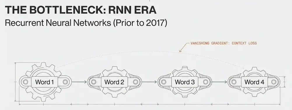
Before 2017, natural language processing relied heavily on Recurrent Neural Networks (RNNs) and their variants (LSTMs, GRUs). These architectures processed text sequentially, maintaining hidden states that captured context:
# Simplified RNN concept
for word in sentence:
    hidden_state = f(hidden_state, word_embedding)
    output = g(hidden_state)
Limitations:
- Sequential processing: No parallelization, slow training.
- Vanishing gradients: Difficulty learning long-range dependencies.
- Limited context: Struggle with sequences longer than ~100-200 tokens.
- Fixed capacity: Hidden state bottleneck.
The “Attention Is All You Need” Breakthrough
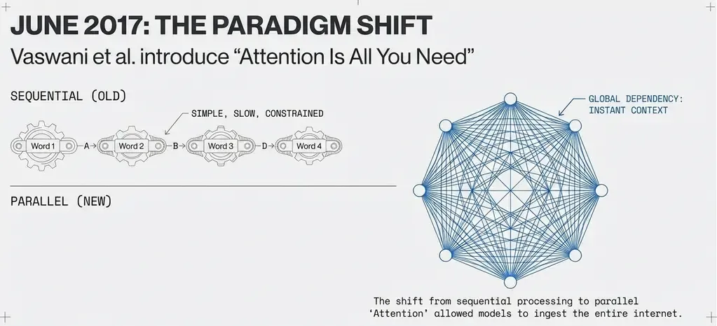
In June 2017, Vaswani et al. published “Attention Is All You Need”, introducing the Transformer architecture that would revolutionize NLP.
Key innovation: Replace sequential processing with parallel attention mechanisms that allow the model to focus on any part of the input simultaneously.
Traditional RNN:  word₁ → word₂ → word₃ → ... → wordₙ  (sequential)

Transformer:      word₁ ↔ word₂ ↔ word₃ ↔ ... ↔ wordₙ  (parallel)
Transformer Architecture: Core Components
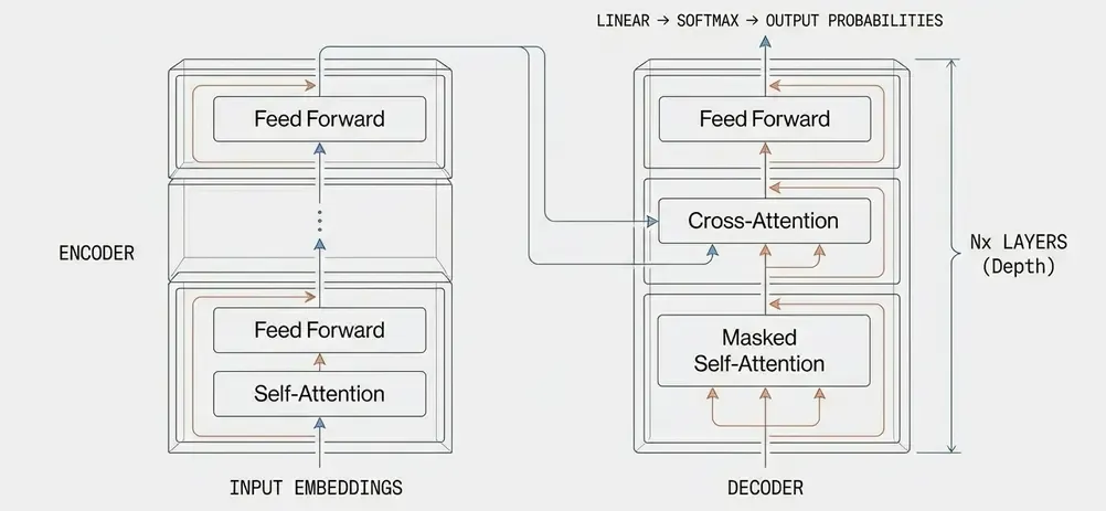
The Transformer consists of two main components: Encoder and Decoder.
High-Level Architecture
Input Text → Tokenization → Embedding → Position Encoding
                                              ↓
                          ┌──────────────────────────────┐
                          │   Encoder Stack (N layers)  │
                          │  - Multi-Head Attention      │
                          │  - Feed Forward Network      │
                          │  - Layer Normalization       │
                          └──────────┬───────────────────┘
                                     ↓
                          ┌──────────────────────────────┐
                          │   Decoder Stack (N layers)  │
                          │  - Masked Multi-Head Attn    │
                          │  - Cross Attention           │
                          │  - Feed Forward Network      │
                          └──────────┬───────────────────┘
                                     ↓
                          Linear → Softmax → Output Token
1. Input Representation
Token Embeddings: Convert discrete tokens to continuous vectors
# Token to embedding
vocab_size = 50000
embedding_dim = 768

embedding_layer = nn.Embedding(vocab_size, embedding_dim)
token_ids = [1234, 5678, 9012]  # "The cat sat"
embeddings = embedding_layer(token_ids)  # Shape: [3, 768]
Positional Encoding: Inject position information (since Transformers have no inherent sequence order)
def positional_encoding(position, d_model):
    """
    PE(pos, 2i)   = sin(pos / 10000^(2i/d_model))
    PE(pos, 2i+1) = cos(pos / 10000^(2i/d_model))
    """
    angle_rates = 1 / np.power(10000, (2 * (np.arange(d_model)//2)) / d_model)
    angle_rads = position * angle_rates

    # Apply sin to even indices, cos to odd
    pe = np.zeros(d_model)
    pe[0::2] = np.sin(angle_rads[0::2])
    pe[1::2] = np.cos(angle_rads[1::2])
    return pe
Self-Attention: The Core Mechanism
Self-attention allows each token to “attend” to all other tokens in the sequence, learning which words are most relevant to each other.
Attention Mathematics
For each token, compute three vectors:
- Query (Q): “What am I looking for?”
- Key (K): “What do I contain?”
- Value (V): “What do I actually represent?”
# Simplified attention computation
def scaled_dot_product_attention(Q, K, V, mask=None):
    """
    Attention(Q, K, V) = softmax(QK^T / √d_k) V
    """
    d_k = Q.size(-1)

    # 1. Compute attention scores
    scores = torch.matmul(Q, K.transpose(-2, -1)) / math.sqrt(d_k)

    # 2. Apply mask (for padding or causal masking)
    if mask is not None:
        scores = scores.masked_fill(mask == 0, -1e9)

    # 3. Softmax to get attention weights
    attention_weights = F.softmax(scores, dim=-1)

    # 4. Apply weights to values
    output = torch.matmul(attention_weights, V)

    return output, attention_weights
Attention Example
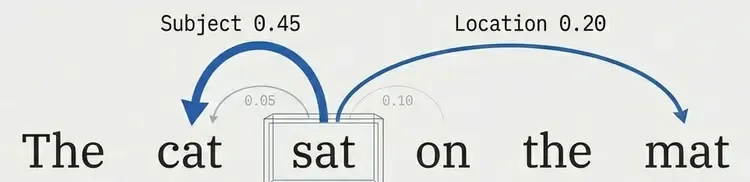
For the sentence “The cat sat on the mat”:
When processing “sat”:
Query: sat
Attention to: The (0.05), cat (0.45), sat (0.10), on (0.15), the (0.05), mat (0.20)
                      ↑ high attention to subject
The model learns that verbs should pay attention to their subjects and objects.
Visualizing Attention
Input:  The    cat    sat    on     the    mat
        ↓      ↓      ↓      ↓      ↓      ↓
Attn:  [0.1]  [0.3]  [0.2]  [0.1]  [0.1]  [0.2]  ← Attention weights for "cat"
        │      │      │      │      │      │
        └──────┴──────┴──────┴──────┴──────┘
                  Weighted combination
                         ↓
                  New representation of "cat"
Multi-Head Attention
Single attention can only learn one type of relationship. Multi-head attention learns multiple relationships in parallel.
class MultiHeadAttention(nn.Module):
    def __init__(self, d_model=768, num_heads=12):
        super().__init__()
        self.num_heads = num_heads
        self.d_model = d_model
        self.d_k = d_model // num_heads

        # Linear projections for Q, K, V
        self.W_q = nn.Linear(d_model, d_model)
        self.W_k = nn.Linear(d_model, d_model)
        self.W_v = nn.Linear(d_model, d_model)
        self.W_o = nn.Linear(d_model, d_model)

    def forward(self, x, mask=None):
        batch_size = x.size(0)

        # 1. Project and split into multiple heads
        Q = self.W_q(x).view(batch_size, -1, self.num_heads, self.d_k).transpose(1, 2)
        K = self.W_k(x).view(batch_size, -1, self.num_heads, self.d_k).transpose(1, 2)
        V = self.W_v(x).view(batch_size, -1, self.num_heads, self.d_k).transpose(1, 2)

        # 2. Apply attention for each head
        attn_output, _ = scaled_dot_product_attention(Q, K, V, mask)

        # 3. Concatenate heads
        attn_output = attn_output.transpose(1, 2).contiguous().view(
            batch_size, -1, self.d_model
        )

        # 4. Final linear projection
        output = self.W_o(attn_output)
        return output
Why multiple heads?
- Head 1: Syntactic relationships (subject-verb).
- Head 2: Semantic similarity (synonyms).
- Head 3: Positional proximity (adjacent words).
- Head 4-12: Other linguistic patterns.
Feed-Forward Networks
After attention, each position passes through a position-wise feed-forward network (FFN):
class FeedForward(nn.Module):
    def __init__(self, d_model=768, d_ff=3072):
        super().__init__()
        self.linear1 = nn.Linear(d_model, d_ff)
        self.linear2 = nn.Linear(d_ff, d_model)
        self.dropout = nn.Dropout(0.1)

    def forward(self, x):
        # FFN(x) = max(0, xW₁ + b₁)W₂ + b₂
return self.linear2(self.dropout(F.gelu(self.linear1(x))))Purpose:
- Non-linear transformation.
- Increase model capacity.
- Learn complex feature interactions.
Layer Normalization and Residual Connections
Residual connections (skip connections) + Layer Normalization stabilize training:
class TransformerBlock(nn.Module):
    def __init__(self, d_model=768, num_heads=12, d_ff=3072):
        super().__init__()
        self.attention = MultiHeadAttention(d_model, num_heads)
        self.feed_forward = FeedForward(d_model, d_ff)
        self.norm1 = nn.LayerNorm(d_model)
        self.norm2 = nn.LayerNorm(d_model)
        self.dropout = nn.Dropout(0.1)

    def forward(self, x, mask=None):
        # 1. Multi-head attention with residual
        attn_output = self.attention(self.norm1(x), mask)
        x = x + self.dropout(attn_output)

        # 2. Feed-forward with residual
        ff_output = self.feed_forward(self.norm2(x))
        x = x + self.dropout(ff_output)

        return x
This pattern is repeated N times (typically 12-96 layers in modern LLMs).
From BERT to GPT: Architectural Variants
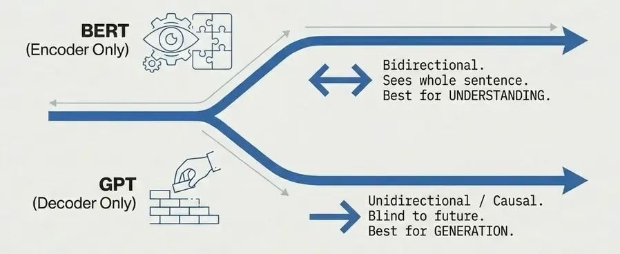
BERT: Bidirectional Encoder (2018)
Architecture: Encoder-only Transformer
[CLS] The cat sat on the mat [SEP]
  ↓    ↓   ↓   ↓   ↓   ↓   ↓    ↓
  ←─────────────────────────────→  Bidirectional attention
  ↓    ↓   ↓   ↓   ↓   ↓   ↓    ↓
 h₁   h₂  h₃  h₄  h₅  h₆  h₇   h₈
Key features:
- Bidirectional context: Each token sees entire sequence.
- Masked Language Modeling (MLM): Predict masked tokens.
- Next Sentence Prediction (NSP): Understand sentence relationships.
Training objective:
# Masked Language Modeling
input_text = "The [MASK] sat on the mat"
target = "cat"

# Model predicts masked token using bidirectional context
prediction = bert(input_text)
loss = cross_entropy(prediction, target)
Use cases:
- Text classification.
- Named entity recognition.
- Question answering.
- Embedding generation.
GPT: Autoregressive Decoder (2018-present)
Architecture: Decoder-only Transformer with causal masking
The    cat    sat    on     the
 ↓      ↓      ↓      ↓      ↓
 →  →→  →→→  →→→→  →→→→→     Causal (left-to-right) attention
 ↓      ↓      ↓      ↓      ↓
 h₁     h₂     h₃     h₄     h₅
Key features:
- Causal attention: Each token only sees previous tokens.
- Autoregressive generation: Predict next token.
- Unidirectional: Left-to-right processing.
Training objective:
# Next Token Prediction
input_text = "The cat sat on"
target = "the"

# Model predicts next token using only previous context
prediction = gpt(input_text)
loss = cross_entropy(prediction, target)
Causal mask implementation:
def create_causal_mask(seq_len):
    """
    Mask out future positions:
    [[1, 0, 0, 0],
     [1, 1, 0, 0],
     [1, 1, 1, 0],
     [1, 1, 1, 1]]
    """
    mask = torch.tril(torch.ones(seq_len, seq_len))
    return mask.view(1, 1, seq_len, seq_len)
Evolution:
- GPT-1 (2018): 117M parameters, proof of concept.
- GPT-2 (2019): 1.5B parameters, coherent text generation.
- GPT-3 (2020): 175B parameters, few-shot learning.
- GPT-3.5 (2022): Optimized for chat, RLHF.
- GPT-4 (2023): Multimodal, enhanced reasoning.
Pre-training vs Fine-tuning
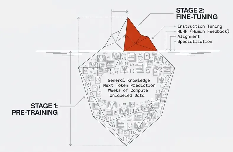
Modern LLMs follow a two-stage training paradigm:
Stage 1: Pre-training
Objective: Learn general language understanding from massive unlabeled data
# Pre-training on raw text
corpus = [
    "The cat sat on the mat.",
    "Natural language processing is fascinating.",
    "Machine learning models require large datasets.",
    # ... billions of sentences
]

# For GPT: predict next token
for text in corpus:
    tokens = tokenize(text)
    for i in range(len(tokens) - 1):
        context = tokens[:i+1]
        target = tokens[i+1]

        prediction = model(context)
        loss = cross_entropy(prediction, target)
        loss.backward()
Data sources:
- Common Crawl (web pages).
- Books (BookCorpus, Books3).
- Wikipedia.
- Scientific papers (arXiv, PubMed).
- Code repositories (GitHub).
Computational requirements:
- GPT-3: ~3.14 × 10²³ FLOPS.
- Training time: Weeks to months on thousands of GPUs.
- Cost: Millions of dollars.
Stage 2: Fine-tuning
Objective: Adapt pre-trained model to specific tasks
# Fine-tuning for specific task
task_data = [
    ("Classify sentiment: I love this product!", "positive"),
    ("Classify sentiment: This is terrible.", "negative"),
    # ... thousands of labeled examples
]

# Fine-tune with task-specific objective
for text, label in task_data:
    prediction = pretrained_model(text)
    loss = task_loss(prediction, label)
    loss.backward()
Fine-tuning approaches:
- Full fine-tuning: Update all parameters.
- Adapter layers: Add small trainable layers, freeze base model.
- LoRA (Low-Rank Adaptation): Efficient parameter updates.
- Prompt tuning: Learn soft prompts, freeze model.
Instruction fine-tuning (modern approach):
instruction_data = [
    {
        "instruction": "Translate to French",
        "input": "Hello, how are you?",
        "output": "Bonjour, comment allez-vous?"
    },
    {
        "instruction": "Summarize this text",
        "input": "Long article text...",
        "output": "Brief summary..."
    }
]
Scaling Laws: Bigger Is Better?
Research shows predictable relationships between model performance and three factors:
The Scaling Laws Formula
Where:
- N: Model size (parameters).
- D: Dataset size (tokens).
- C: Compute budget (FLOPs).
- α, β, γ: Empirically determined exponents.
Key Findings
- Performance scales predictably with size.
- Compute is the limiting factor, not parameters or data.
- Optimal allocation:
- Double compute → 1.7× larger model + 1.2× more data.
- Diminishing returns but no clear saturation point yet.
Model Size Evolution
| Model | Year | Parameters | Training Tokens |
|---|---|---|---|
| BERT-Base | 2018 | 110M | ~3B |
| GPT-2 | 2019 | 1.5B | ~40B |
| GPT-3 | 2020 | 175B | ~300B |
| Gopher | 2021 | 280B | ~300B |
| PaLM | 2022 | 540B | ~780B |
| LLaMA | 2023 | 65B | ~1.4T |
| GPT-4 | 2023 | ~1.7T* | Unknown |
*Rumored, not confirmed
Emergent Abilities
As models scale, they exhibit emergent abilities: capabilities not present in smaller models that suddenly appear at certain scale thresholds.
Examples of Emergence
- Few-shot learning: Learn from examples without fine-tuning.
- Chain-of-thought reasoning: Break down complex problems.
- Code generation: Write functional programs.
- Multi-step math: Solve complex calculations.
- Translation: Even for low-resource language pairs.
Scaling Curve Example
Performance on Complex Task
    │
100%│                              ┌────
    │                            ╱
 75%│                          ╱
    │                        ╱
 50%│                    ╱╱
    │              ╱╱╱╱
 25%│      ╱╱╱╱╱╱
    │╱╱╱╱╱
  0%└──────────────────────────────────
    1M   10M  100M   1B   10B  100B  1T
              Model Parameters
Emergence threshold: Often around 10B-100B parameters for complex reasoning tasks.
Training Techniques
1. Mixed Precision Training
Use FP16/BF16 for speed, FP32 for stability:
from torch.cuda.amp import autocast, GradScaler

scaler = GradScaler()

for batch in dataloader:
    with autocast():
        output = model(batch)
        loss = criterion(output, target)

    scaler.scale(loss).backward()
    scaler.step(optimizer)
    scaler.update()
2. Gradient Checkpointing
Trade compute for memory:
# Store only some activations, recompute others during backward
from torch.utils.checkpoint import checkpoint

def forward(self, x):
    for layer in self.layers:
        x = checkpoint(layer, x)  # Recompute instead of storing
    return x
3. Model Parallelism
Split model across multiple GPUs:
- Pipeline parallelism: Different layers on different GPUs.
- Tensor parallelism: Split individual layers.
- Data parallelism: Replicate model, split data.
4. Optimizer Improvements
AdamW (Adam with decoupled weight decay):
optimizer = torch.optim.AdamW(
    model.parameters(),
    lr=1e-4,
    betas=(0.9, 0.999),
    weight_decay=0.01
)
Learning rate schedule:
# Warmup + Cosine decay
def get_lr(step, warmup_steps, total_steps, max_lr):
    if step < warmup_steps:
        return max_lr * step / warmup_steps
    else:
        progress = (step - warmup_steps) / (total_steps - warmup_steps)
        return max_lr * 0.5 * (1 + math.cos(math.pi * progress))
Tokenization
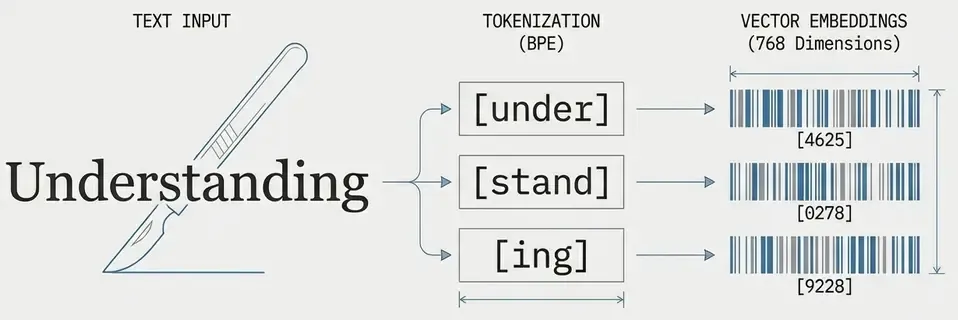
Before processing, text must be converted to tokens. Modern LLMs use subword tokenization.
Byte-Pair Encoding (BPE)
Most common approach (used by GPT):
# Example tokenization
text = "understanding"

# Character level: ["u", "n", "d", "e", "r", "s", "t", "a", "n", "d", "i", "n", "g"]
# Subword level: ["under", "stand", "ing"]
# Word level: ["understanding"]

# GPT tokenization
from transformers import GPT2Tokenizer
tokenizer = GPT2Tokenizer.from_pretrained("gpt2")

tokens = tokenizer.encode("understanding")
# Output: [4625, 278, 9228]  (approximate)
Advantages:
- Balance between vocabulary size and sequence length.
- Handle rare words and typos.
- Efficient for multiple languages.
Vocabulary sizes:
- GPT-2/GPT-3: ~50k tokens.
- LLaMA: ~32k tokens.
- GPT-4: ~100k tokens (estimated).
Architecture Comparison Summary
| Aspect | BERT | GPT | T5 |
|---|---|---|---|
| Type | Encoder-only | Decoder-only | Encoder-Decoder |
| Attention | Bidirectional | Causal (unidirectional) | Both |
| Training | MLM + NSP | Next token prediction | Span corruption |
| Best for | Understanding | Generation | Translation, summarization |
| Context | Full sequence | Left-to-right | Input→Output |
Computational Considerations
Model Size vs Memory
For a model with N parameters:
- Storage: ~4N bytes (FP32) or ~2N bytes (FP16).
- Training memory: ~16-20N bytes (gradients, optimizer states, activations).
- Inference memory: ~4-8N bytes.
Example: GPT-3 175B:
- Storage: ~350 GB (FP16).
- Training: ~3 TB.
- Inference: ~700 GB.
Inference Optimization
- Quantization: Reduce precision (INT8, INT4).
- Pruning: Remove unnecessary weights.
- Distillation: Train smaller model to mimic larger one.
- KV caching: Store attention keys/values for faster generation.
# KV caching for autoregressive generation
cache = {}
for position in range(max_length):
    # Reuse previous computations
    output, cache = model(input, cache=cache)
    next_token = sample(output)
    input = torch.cat([input, next_token])
Limitations and Challenges
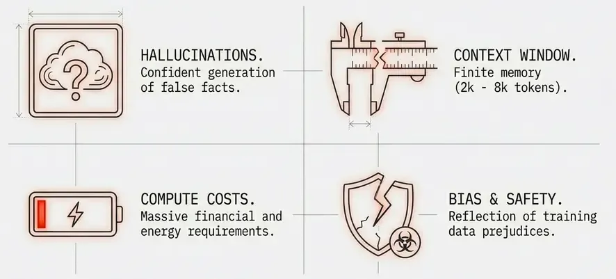
1. Training Costs
- Compute: Millions of dollars for large models.
- Energy: Environmental concerns.
- Accessibility: Only large organizations can train from scratch.
2. Context Length
- Limited window: Most models handle 2k-8k tokens.
- Information loss: Can’t process very long documents.
- Workarounds: Chunking, summarization, retrieval.
3. Hallucinations
- Confident but wrong: Generate plausible-sounding false information.
- No grounding: No connection to real-world facts.
- Mitigation: Retrieval augmentation, fact-checking.
4. Bias and Safety
- Training data bias: Reflect biases in training data.
- Harmful content: Can generate toxic or dangerous text.
- Alignment: Ensuring models behave as intended.
The Future: What’s Next?
Emerging Trends
-
Efficient architectures:
- Sparse attention mechanisms.
- State space models (S4, Mamba).
- Mixture of Experts (MoE).
-
Longer context:
- Efficient attention variants (Linear attention, Flash attention).
- Retrieval augmentation.
- Memory mechanisms.
-
Multimodal models:
- Vision + Language (CLIP, Flamingo).
- Audio + Language.
- Video understanding.
-
Smaller, efficient models:
- Distillation techniques.
- Efficient fine-tuning (LoRA, QLoRA).
- On-device models.
-
Better training methods:
- Improved data quality.
- Curriculum learning.
- Multi-task learning.
Conclusion
Large Language Models represent a paradigm shift in how we build AI systems. The Transformer architecture’s ability to process language in parallel, combined with self-attention mechanisms and massive scale, has unlocked capabilities that were unimaginable just a few years ago.
Key takeaways:
- Transformers replaced RNNs through parallel processing and attention.
- Self-attention allows models to learn complex relationships in text.
- Scaling laws show predictable improvements with size and compute.
- Pre-training + fine-tuning enables transfer learning at massive scale.
- Emergent abilities appear at certain scale thresholds.
- Architecture choices (encoder vs decoder) determine capabilities.
Understanding these fundamentals is crucial for anyone working with modern AI systems. As we continue to push the boundaries of scale and capability, these core principles remain the foundation upon which all LLM applications are built.
In future posts, we’ll explore how to leverage these models in production systems, from embeddings and semantic search to retrieval-augmented generation and beyond.
References
- Vaswani et al. (2017): “Attention Is All You Need”
- Devlin et al. (2018): “BERT: Pre-training of Deep Bidirectional Transformers”
- Radford et al. (2018): “Improving Language Understanding by Generative Pre-Training”
- Brown et al. (2020): “Language Models are Few-Shot Learners” (GPT-3)
- Kaplan et al. (2020): “Scaling Laws for Neural Language Models”
- Wei et al. (2022): “Emergent Abilities of Large Language Models”
- Hoffmann et al. (2022): “Training Compute-Optimal Large Language Models” (Chinchilla)